Structured Streaming Programming Guide
Quick Example
Let’s say you want to maintain a running word count of text data received from a data server listening on a TCP socket. Let’s see how you can express this using Structured Streaming. You can see the full code in Python/Scala/Java/R. And if you download Spark, you can directly run the example. In any case, let’s walk through the example step-by-step and understand how it works. First, we have to import the necessary classes and create a local SparkSession, the starting point of all functionalities related to Spark.
from pyspark.sql import SparkSession
from pyspark.sql.functions import explode
from pyspark.sql.functions import split

spark = SparkSession \
    .builder \
    .appName("StructuredNetworkWordCount") \
    .getOrCreate()
import org.apache.spark.sql.functions._
import org.apache.spark.sql.SparkSession
val spark = SparkSession
.builder
.appName("StructuredNetworkWordCount")
.getOrCreate()
import spark.implicits._import org.apache.spark.api.java.function.FlatMapFunction;
import org.apache.spark.sql.*;
import org.apache.spark.sql.streaming.StreamingQuery;
import java.util.Arrays;
import java.util.Iterator;
SparkSession spark = SparkSession
.builder()
.appName("JavaStructuredNetworkWordCount")
.getOrCreate();sparkR.session(appName = "StructuredNetworkWordCount")Next, let’s create a streaming DataFrame that represents text data received from a server listening on localhost:9999, and transform the DataFrame to calculate word counts.
# Create DataFrame representing the stream of input lines from connection to localhost:9999
lines = spark \
    .readStream \
    .format("socket") \
    .option("host", "localhost") \
    .option("port", 9999) \
    .load()

# Split the lines into words
words = lines.select(
   explode(
       split(lines.value, " ")
   ).alias("word")
)

# Generate running word count
wordCounts = words.groupBy("word").count()
This lines DataFrame represents an unbounded table containing the streaming text data. This table contains one column of strings named “value”, and each line in the streaming text data becomes a row in the table. Note, that this is not currently receiving any data as we are just setting up the transformation, and have not yet started it. Next, we have used two built-in SQL functions - split and explode, to split each line into multiple rows with a word each. In addition, we use the function alias to name the new column as “word”. Finally, we have defined the wordCounts DataFrame by grouping by the unique values in the Dataset and counting them. Note that this is a streaming DataFrame which represents the running word counts of the stream.
// Create DataFrame representing the stream of input lines from connection to localhost:9999
val lines = spark.readStream
  .format("socket")
  .option("host", "localhost")
  .option("port", 9999)
  .load()

// Split the lines into words
val words = lines.as[String].flatMap(_.split(" "))

// Generate running word count
val wordCounts = words.groupBy("value").count()
This lines DataFrame represents an unbounded table containing the streaming text data. This table contains one column of strings named “value”, and each line in the streaming text data becomes a row in the table. Note, that this is not currently receiving any data as we are just setting up the transformation, and have not yet started it. Next, we have converted the DataFrame to a Dataset of String using .as[String], so that we can apply the flatMap operation to split each line into multiple words. The resultant words Dataset contains all the words. Finally, we have defined the wordCounts DataFrame by grouping by the unique values in the Dataset and counting them. Note that this is a streaming DataFrame which represents the running word counts of the stream.
// Create DataFrame representing the stream of input lines from connection to localhost:9999
Dataset<Row> lines = spark
  .readStream()
  .format("socket")
  .option("host", "localhost")
  .option("port", 9999)
  .load();

// Split the lines into words
Dataset<String> words = lines
  .as(Encoders.STRING())
  .flatMap((FlatMapFunction<String, String>) x -> Arrays.asList(x.split(" ")).iterator(), Encoders.STRING());

// Generate running word count
Dataset<Row> wordCounts = words.groupBy("value").count();
This lines DataFrame represents an unbounded table containing the streaming text data. This table contains one column of strings named “value”, and each line in the streaming text data becomes a row in the table. Note, that this is not currently receiving any data as we are just setting up the transformation, and have not yet started it. Next, we have converted the DataFrame to a Dataset of String using .as(Encoders.STRING()), so that we can apply the flatMap operation to split each line into multiple words. The resultant words Dataset contains all the words. Finally, we have defined the wordCounts DataFrame by grouping by the unique values in the Dataset and counting them. Note that this is a streaming DataFrame which represents the running word counts of the stream.
# Create DataFrame representing the stream of input lines from connection to localhost:9999
lines <- read.stream("socket", host = "localhost", port = 9999)

# Split the lines into words
words <- selectExpr(lines, "explode(split(value, ' ')) as word")

# Generate running word count
wordCounts <- count(group_by(words, "word"))
This lines SparkDataFrame represents an unbounded table containing the streaming text data. This table contains one column of strings named “value”, and each line in the streaming text data becomes a row in the table. Note, that this is not currently receiving any data as we are just setting up the transformation, and have not yet started it. Next, we have a SQL expression with two SQL functions - split and explode, to split each line into multiple rows with a word each. In addition, we name the new column as “word”. Finally, we have defined the wordCounts SparkDataFrame by grouping by the unique values in the SparkDataFrame and counting them. Note that this is a streaming SparkDataFrame which represents the running word counts of the stream.
We have now set up the query on the streaming data. All that is left is to actually start receiving data and computing the counts. To do this, we set it up to print the complete set of counts (specified by outputMode("complete")) to the console every time they are updated. And then start the streaming computation using start().
 # Start running the query that prints the running counts to the console
query = wordCounts \
    .writeStream \
    .outputMode("complete") \
    .format("console") \
    .start()

query.awaitTermination()
// Start running the query that prints the running counts to the console
val query = wordCounts.writeStream
.outputMode("complete")
.format("console")
.start()
query.awaitTermination()// Start running the query that prints the running counts to the console
StreamingQuery query = wordCounts.writeStream()
.outputMode("complete")
.format("console")
.start();
query.awaitTermination();# Start running the query that prints the running counts to the console
query <- write.stream(wordCounts, "console", outputMode = "complete")
awaitTermination(query)After this code is executed, the streaming computation will have started in the background. The query object is a handle to that active streaming query, and we have decided to wait for the termination of the query using awaitTermination() to prevent the process from exiting while the query is active.
To actually execute this example code, you can either compile the code in your own Spark application, or simply run the example once you have downloaded Spark. We are showing the latter. You will first need to run Netcat (a small utility found in most Unix-like systems) as a data server by using
$ nc -lk 9999
Then, in a different terminal, you can start the example by using
$ ./bin/spark-submit examples/src/main/python/sql/streaming/structured_network_wordcount.py localhost 9999$ ./bin/run-example org.apache.spark.examples.sql.streaming.StructuredNetworkWordCount localhost 9999$ ./bin/run-example org.apache.spark.examples.sql.streaming.JavaStructuredNetworkWordCount localhost 9999$ ./bin/spark-submit examples/src/main/r/streaming/structured_network_wordcount.R localhost 9999Then, any lines typed in the terminal running the netcat server will be counted and printed on screen every second. It will look something like the following.
|
|
Programming Model
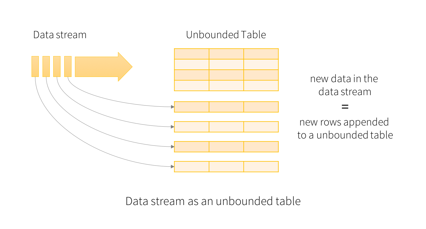
The key idea in Structured Streaming is to treat a live data stream as a table that is being continuously appended. This leads to a new stream processing model that is very similar to a batch processing model. You will express your streaming computation as standard batch-like query as on a static table, and Spark runs it as an incremental query on the unbounded input table. Let’s understand this model in more detail.
Basic Concepts
Consider the input data stream as the “Input Table”. Every data item that is arriving on the stream is like a new row being appended to the Input Table.

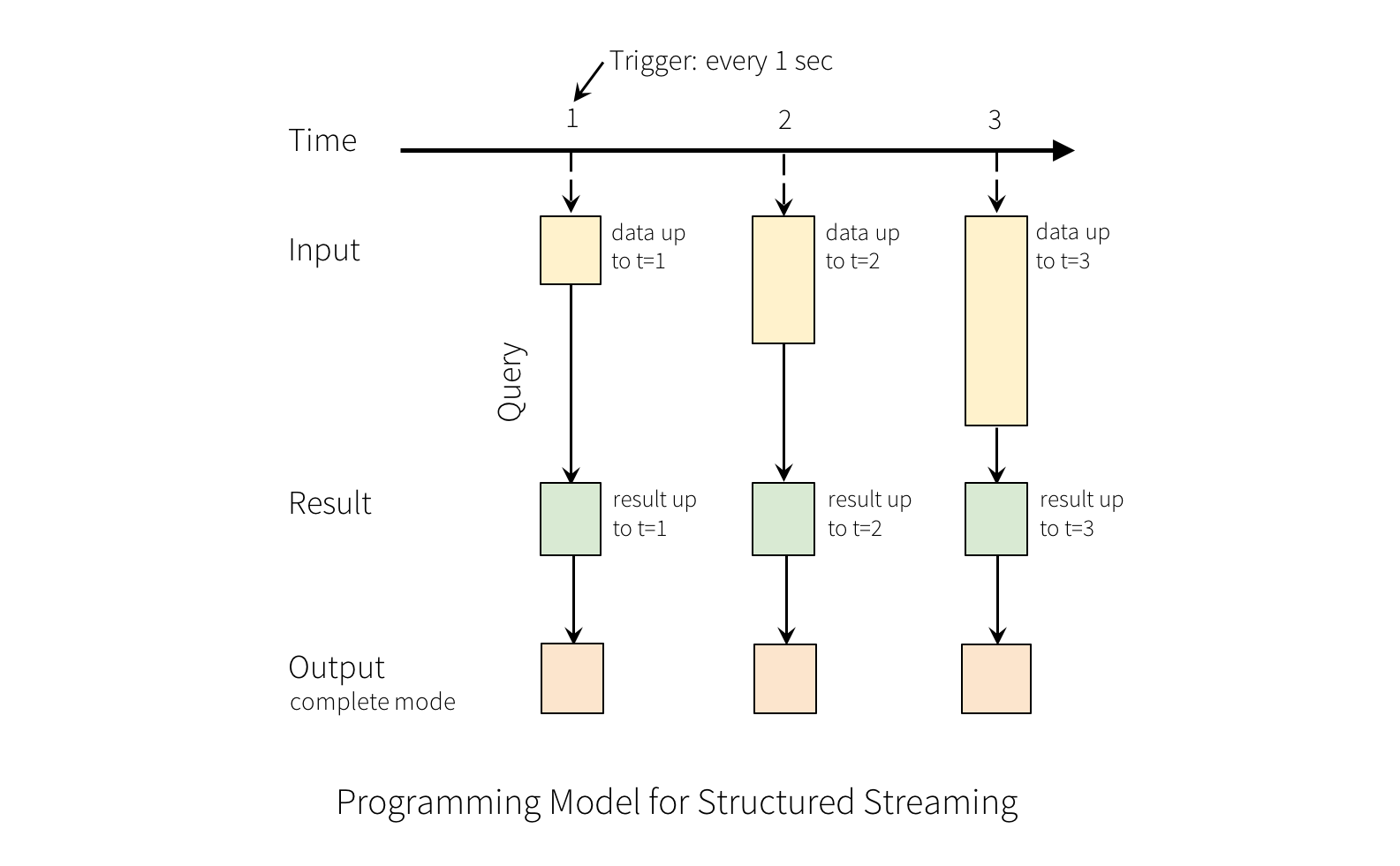
A query on the input will generate the “Result Table”. Every trigger interval (say, every 1 second), new rows get appended to the Input Table, which eventually updates the Result Table. Whenever the result table gets updated, we would want to write the changed result rows to an external sink.

The “Output” is defined as what gets written out to the external storage. The output can be defined in a different mode:
-
Complete Mode - The entire updated Result Table will be written to the external storage. It is up to the storage connector to decide how to handle writing of the entire table.
-
Append Mode - Only the new rows appended in the Result Table since the last trigger will be written to the external storage. This is applicable only on the queries where existing rows in the Result Table are not expected to change.
-
Update Mode - Only the rows that were updated in the Result Table since the last trigger will be written to the external storage (available since Spark 2.1.1). Note that this is different from the Complete Mode in that this mode only outputs the rows that have changed since the last trigger. If the query doesn’t contain aggregations, it will be equivalent to Append mode.
Note that each mode is applicable on certain types of queries. This is discussed in detail later.
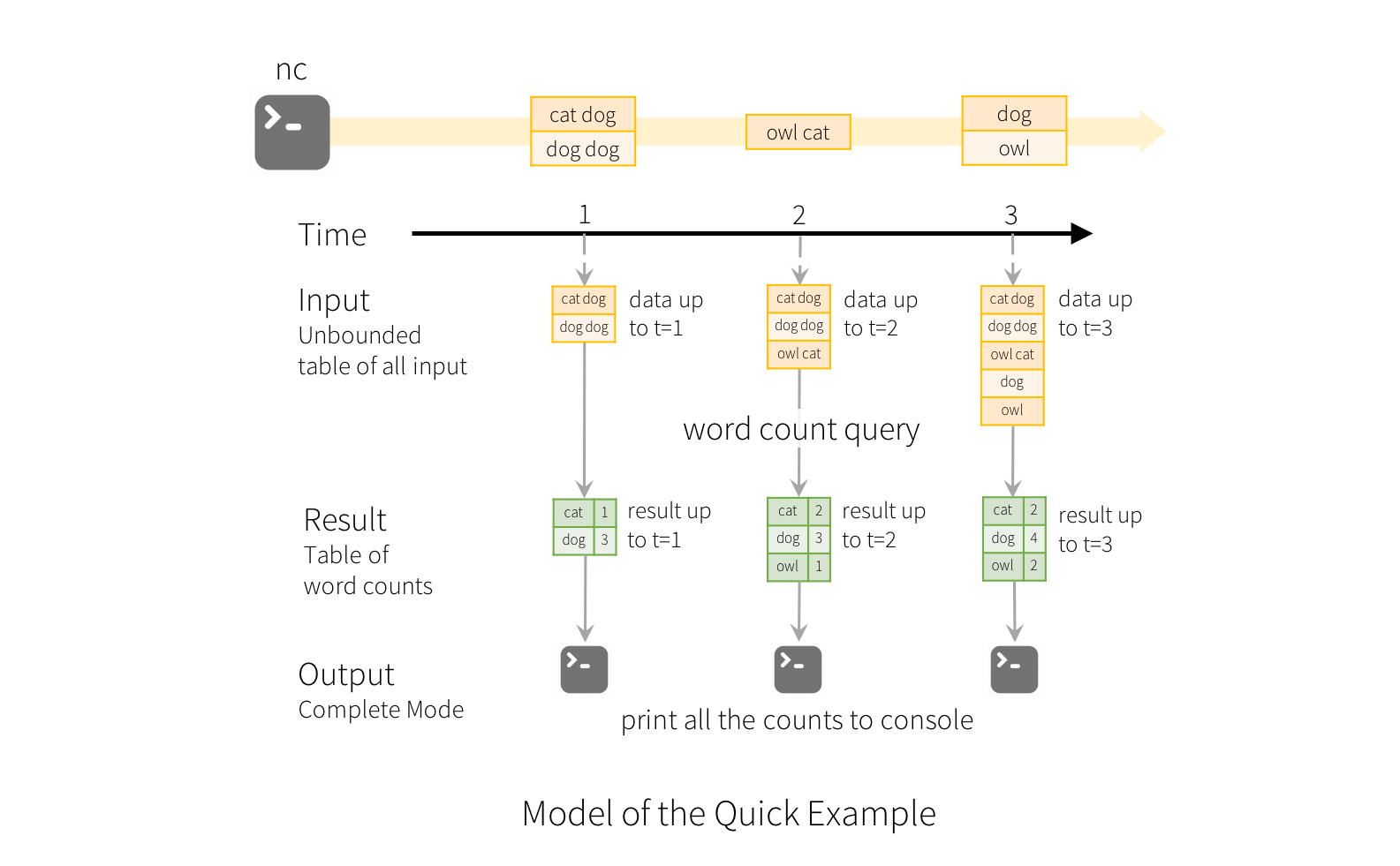
To illustrate the use of this model, let’s understand the model in context of
the Quick Example above. The first lines DataFrame is the input table, and
the final wordCounts DataFrame is the result table. Note that the query on
streaming lines DataFrame to generate wordCounts is exactly the same as
it would be a static DataFrame. However, when this query is started, Spark
will continuously check for new data from the socket connection. If there is
new data, Spark will run an “incremental” query that combines the previous
running counts with the new data to compute updated counts, as shown below.

Note that Structured Streaming does not materialize the entire table. It reads the latest available data from the streaming data source, processes it incrementally to update the result, and then discards the source data. It only keeps around the minimal intermediate state data as required to update the result (e.g. intermediate counts in the earlier example).
This model is significantly different from many other stream processing engines. Many streaming systems require the user to maintain running aggregations themselves, thus having to reason about fault-tolerance, and data consistency (at-least-once, or at-most-once, or exactly-once). In this model, Spark is responsible for updating the Result Table when there is new data, thus relieving the users from reasoning about it. As an example, let’s see how this model handles event-time based processing and late arriving data.
Handling Event-time and Late Data
Event-time is the time embedded in the data itself. For many applications, you may want to operate on this event-time. For example, if you want to get the number of events generated by IoT devices every minute, then you probably want to use the time when the data was generated (that is, event-time in the data), rather than the time Spark receives them. This event-time is very naturally expressed in this model – each event from the devices is a row in the table, and event-time is a column value in the row. This allows window-based aggregations (e.g. number of events every minute) to be just a special type of grouping and aggregation on the event-time column – each time window is a group and each row can belong to multiple windows/groups. Therefore, such event-time-window-based aggregation queries can be defined consistently on both a static dataset (e.g. from collected device events logs) as well as on a data stream, making the life of the user much easier.
Furthermore, this model naturally handles data that has arrived later than expected based on its event-time. Since Spark is updating the Result Table, it has full control over updating old aggregates when there is late data, as well as cleaning up old aggregates to limit the size of intermediate state data. Since Spark 2.1, we have support for watermarking which allows the user to specify the threshold of late data, and allows the engine to accordingly clean up old state. These are explained later in more detail in the Window Operations section.
Fault Tolerance Semantics
Delivering end-to-end exactly-once semantics was one of key goals behind the design of Structured Streaming. To achieve that, we have designed the Structured Streaming sources, the sinks and the execution engine to reliably track the exact progress of the processing so that it can handle any kind of failure by restarting and/or reprocessing. Every streaming source is assumed to have offsets (similar to Kafka offsets, or Kinesis sequence numbers) to track the read position in the stream. The engine uses checkpointing and write-ahead logs to record the offset range of the data being processed in each trigger. The streaming sinks are designed to be idempotent for handling reprocessing. Together, using replayable sources and idempotent sinks, Structured Streaming can ensure end-to-end exactly-once semantics under any failure.